
Back in 2006, Netflix issued a challenge to predict user scores of movies given the user’s past ratings and ratings of other users. In other words, Netflix provided 100M ratings of 17K movies by 500K users and asked to fill in certain cells, as shown in the image below. The difficulty in their provided data was that only 100M ratings were present out of 8.5B possible entries. Simon Funk used a singular value decomposition (SVD) approach that got him 3rd place in the challenge. In this post, we explore the method and math of his approach and then implement it on a toy problem using Tensorflow. In the next post, I will apply the method to real data. If you’re interested in the original post by Simon Funk, check his blog here: link.
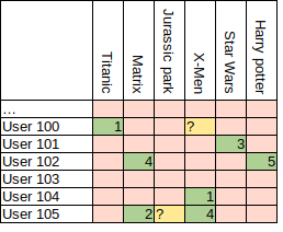
Ratings are sparsely populated in 1 to 5 range. Question marks need to be filled.
Filling out this matrix, or certain cells, is useful for recommendation systems. If we can figure out a good method to fill the matrix, then we simply look up a rating for any movie for any new user. I decided to make this post because I found the method quite interesting to study. As we will see soon, the method is based on gradient descent, which means we can use Tensorflow to implement it. If you’re interested in Funk’s method or you’re not familiar with how to write custom training loops in Tensorflow, you might learn something. Or not.
The post will go as follows:
- Introduction to method and math
- Writing a basic implementation in Tensorflow
- Applying the method to a toy problem
- Applying the method to real data. – This one is cover in the next post.
Introduction
The method applies an SVD decomposition to the given giant matrix. The SVD decomposition of any matrix can be written as: A = U S VT, where U and V are ortho-normal matrices, shown below. In fact, if you’re familiar with PCA, the columns of V are the principal axes of PCA. S is a diagonal matrix.

SVD decomposition. Image from Wikipedia. By Cmglee – Own work, CC BY-SA 4.0, https://commons.wikimedia.org/w/index.php?curid=67853297
It would appear that the SVD decomposition of a matrix is actually larger than the original matrix. However, theory states that if you cut off the decomposition to some row and column k, then that decomposition will be the best approximation of the original matrix. Then, the decomposition that Funk proposed was M = U500,000×40 V40×17,000, roughly shown below. We assume that the diagonal matrix that appears in the middle has been multiplied into either U or V.

Funk’s SVD decomposition of Netflix ranking matrix
The intuition behind this decomposition is that many users will have typical ranking patterns. For example, action movie fans will rank action movies high and romance movies low. This means that we can classify users into what kind of movie fan that person is and that classification requires not that many parameters. Thus, each 40 dimensional column vector of VT assigns a latent space representation of each user. In a similar manner, any movie can also be encoded into a latent representation, given as a 40 dimensional row vector of U. However, the row vectors of U does not have an intuitive explanation, as they are completely tied with column vectors of V to give movie rankings.
The question is then how to determine the rows and columns of U and V. This is done simply by initializing random U and V matrices and then performing gradient descent until the original M matrix is approximated. The ranking of i’th movie by j’th user can be predicted as:
Where ui is the i’th row of U and vj is the j’th column of V. The error between the prediction and the real matrix value can then be written as:

We can then define a full loss function as the MSE between prediction and corresponding entries in the matrix M as:

Our goal is to minimize L with respect to the entries of U and V. This is a familiar problem definition for people who has done neural network training. We can write down the weights update step as:

Since the problem is symmetric, for U and V, the u‘s and v‘s in the equation above can be replaced to obtain the update step for v‘s.
One important thing to mention is that the original M matrix is very sparsely populated. To get around this problem, we simply ignore cells that don’t have any ranking and only train on available rankings. The hope is that this will still allow us to obtain a good latent representation through U and V.
Basic Implementation in Tensorflow
With the theory out of the way, now we can implement this in Tensorflow. In this section, I will only write a simple training loop for some arbitrary matrix. For this step, we will generate the matrix M from known U and V matrices. Then, we try to estimate U and V using gradient descent.
import numpy as np
import matplotlib.pyplot as plt
import tensorflow as tf

#uncomment this if you're using jupyter notebook
#%matplotlib inline

#generate known U and V matrices
U = tf.random.normal((3,3), dtype = 'float32')
V = tf.random.normal((3,3), dtype = 'float32')

#Our (3,3) "ranking" matrix.
M = U @ V

#we can visualize what our matrices look like
plt.subplot(131)
plt.imshow(U)
plt.subplot(132)
plt.imshow(V)
plt.subplot(133)
plt.imshow(T)
plt.show()

M = U x V
Next, we create random matrices for U and V. These we hope will eventually become U and V. If you’re not familiar with tensorflow, tensors that you want to take derivative with needs to be initialized with tf.Variable(). Otherwise, non-changing tensors are generated with tf.constant().
U_d = tf.Variable(tf.random.normal((3,3), dtype = 'float32'))
V_d = tf.Variable(tf.random.normal((3,3), dtype = 'float32'))
Now we can write the basic training loop. The nice perk of using tensorflow is that the update step equations I wrote above is automatically taken care of by tensorflow. Here I use the vanilla gradient descent step, as was done by Funk in 2006.
epochs = 10000
lr = 0.001
losses = []

for ep in range(epochs):

    with tf.GradientTape() as tape:
        M_app = U_d @ V_d
        loss = tf.reduce_mean(tf.square(M - M_app))

    losses.append(loss.numpy())
    grads = tape.gradient(loss, [U_d, V_d])

    U_d.assign_sub(lr * grads[0])
    V_d.assign_sub(lr * grads[1])

losses = np.array(losses)
plt.plot(losses)
plt.title('loss')
plt.xlabel('step')
plt.show()

Loss function of training.
We see that our approximated U and V matrices produce very small loss. After 10,000 training iterations, I get an average difference of 0.006 MSE, or 0.077 real difference. This is not bad. However, it took us about 10,000 iterations to get here. We can apply some modernization to the training loop by switching to the Adam optimizer. If you increase the size of U and V to 500×500, then using vanilla gradient descent will take over an hour and more than 3 million training iterations to get to under 0.01 MSE. Adam will do it in about 4 seconds and 2000 iterations. In any case, Adam can be added to the training loop with only 2 lines.
U_d = tf.Variable(tf.random.normal((3,3), dtype = 'float32'))
V_d = tf.Variable(tf.random.normal((3,3), dtype = 'float32'))
adam_opt = tf.keras.optimizers.Adam(lr = 0.01)

epochs = 200
losses_adam = []

for ep in range(epochs):

    with tf.GradientTape() as tape:
        M_app = U_d @ V_d
        loss = tf.reduce_mean(tf.square(M - M_app))

    print(ep, loss)
    losses_adam.append(loss.numpy())
    grads = tape.gradient(loss, [U_d, V_d])
    adam_opt.apply_gradients(zip(grads, [U_d, V_d]))

plt.plot(losses_adam, label = 'adam_loss')
plt.plot(losses, label = 'loss GD')
plt.legend()
plt.show()

Comparison of Adam and vanilla GD.
Finally we check if the original U and V are the same as the approximated U and V. In general, we should not expect them to be the same. Can you reason out why? We can plot U and V matrices side by side to see the difference.
M_app = U_d @ V_d
plt.figure(figsize=(12,16))
plt.subplot(321)
plt.imshow(U)
plt.title('U original')
plt.subplot(322)
plt.imshow(U_d.numpy())
plt.title('U from tensorflow')
plt.subplot(323)
plt.imshow(V)
plt.title('V original')
plt.subplot(324)
plt.imshow(V_d.numpy())
plt.title('V from tensorflow')
plt.subplot(325)
plt.imshow(M)
plt.title('M original')
plt.subplot(326)
plt.imshow(M_app.numpy())
plt.title('M from tensorflow')
plt.show()

Comparison of original U,V and M matrices with those determined by tensorflow.
We can see that the U and V matrices determined by tensorflow are completely different from the original matrices used to generate M. But the matrix M determined by multiplying U_d and V_d are very close to the original. The reason why this happens is because we only constrain the dot products of rows of U and columns of V to be equal to the corresponding entry in M. We don’t actually constrain the row and column vectors of U and V themselves. Another way to think about this is that dot product is rotation invariant. So if we apply rotational coordinate transform to the rows and columns of U and V, we get different vectors but the dot product is still the same.
So with this simple exercise, we find that the U and V decomposition of M can be found with gradient descent algorithm in tensorflow. If you want, you can increase the size of generating U and V matrices and watch your computer crunch through a relatively boring computation.
Applying the Funk SVD to a Toy Problem
Now we want to apply the SVD decomposition to a toy problem. Our goal is to generate a large matrix M from U and V and then try to approximate M using a much smaller U_d and V_d matrices. For this to work, we need to make sure that the matrix M actually can be represented by fewer vectors than the full rows and columns of U and V. To ensure this, we simply weight the generating products by the harmonic series. Note that when generating the matrix M, we are taking the outer product of the columns of U and rows of V, which is not how we usually take the product of two matrices. This simply allows us to weight the contribution of each column and row of U and V.
import tensorflow as tf
import numpy as np
import matplotlib.pyplot as plt

#uncomment this if not using jupyter notebook
%matplotlib inline

U = tf.random.normal((500,500), dtype = 'float32')
V = tf.random.normal((500,500), dtype = 'float32')

T = tf.zeros((500,500), dtype = 'float32')
for i in range(U.shape[0]):
    T = T + 1/(i + 1) * (U[:,i:i+1] @ V[i:i+1,:])

harm = np.array([1/(i + 1) for i in range(500) ])
plt.plot(harm)
plt.show()

Harmonic series weighting. We see that only the first 50 or columns and rows of U and V contribute to M. The rest contribute insignificantly.
Next we randomly remove entries from the matrix M. Remember that in the original Netflix matrix, only 100M were filled out of 8.5B. In this toy example, we can tune how much of the original matrix to mask out with the variable sparcity_ratio. Also I’ve misspelled sparsity but too lazy to modify my code.
#adding a sparcity mask
sparcity_mat = np.ones((500,500))

#How much of the matrix to mask. This is not strictly kept as some random indices will coincide
sparcity_ratio = .7
i = np.random.randint(0, M.shape[0], int(sparcity_ratio * M.shape[0] * M.shape[1]))
j = np.random.randint(0, M.shape[1], int(sparcity_ratio * M.shape[0] * M.shape[1]))
sparcity_mat[i,j] = 0

sparcity_mat = tf.constant(sparcity_mat, dtype = 'float32')
print('nonzero entries ratio: ', (tf.reduce_sum(sparcity_mat)/(sparcity_mat.shape[0] * sparcity_mat.shape[1])).numpy())

#this matrix contains 1's where we have masked
masked_entries = tf.cast(tf.not_equal(sparcity_mat, 1), dtype = 'float32')
Using a ratio of 0.7 masks out about 50% of the matrix M. For now, we only obtain sparcity_mat and masked_entries. These are binary masks that we can multiply to M and obtain the masked and unmasked parts of M. We can also visualize what our masking looks like.
plt.figure(figsize=(8,8))
plt.imshow(sparcity_mat)
plt.show()
![]()
Dots represent entries that remain in M. The blanks represent the entries that we removed from M. Our goal is to estimate these blank spots after U and V decomposition.
I’ve also added a small function that stops training if validation loss remains that same or starts to increase.
def early_stopping(losses, patience = 5):

    if len(losses) <= patience + 1:
        return False

    avg_loss = np.mean(losses[-1 - patience:-1])

    if avg_loss - losses[-1] < 0.01*avg_loss:
        return True

    return False
We can now apply the SVD decomposition method from last step to this new sparse matrix. We generated M from U and V matrix with dimensions (500×500). Here we try to approximate it with a (500×30) and (30×500) matrices. We also use the masked parts of the M matrix as our validation set. Our main goal is to approximate these masked entries. So the loss function of this validation set is the most important, as it measures how good we are at predicting these unknowns.
U_d = tf.Variable(tf.random.normal((500, 30)))
V_d = tf.Variable(tf.random.normal((30, 500)))
adam_opt = tf.keras.optimizers.Adam()

from datetime import datetime
ep = 0
start_time = datetime.now()

losses = []
val_losses = []

#normalization factors for training entries and validation entries.
train_norm = tf.reduce_sum(sparcity_mat)
val_norm = tf.reduce_sum(masked_entries)

while True:

    with tf.GradientTape() as tape:
        M_app = U_d @ V_d

        pred_errors_squared = tf.square(M - M_app)
        loss = tf.reduce_sum((sparcity_mat * pred_errors_squared)/train_norm)

    val_loss = tf.reduce_sum((masked_entries * pred_errors_squared)/val_norm)

    if ep%1000 == 0:
        print(datetime.now() - start_time, loss, val_loss, ep)
        losses.append(loss.numpy())
        val_losses.append(val_loss.numpy())
    if early_stopping(val_losses):
        break

    grads = tape.gradient(loss, [U_d, V_d])
    adam_opt.apply_gradients(zip(grads, [U_d, V_d]))

    ep += 1

print('total time: ', datetime.now() - start_time)
print('epochs: ', ep)

Validation and training loss
My GTX1080 GPU ran through 21,000 iterations in about 40 seconds and obtained a validation loss of 0.032 MSE, or 0.17 mean error. Is this good? Our M matrix is generated by sampling from a Gaussian centered around 0 and stddev of 1. So M matrix has entries in the range of about [-2, 2]. An average error of 0.17 is not that good but not that bad. More importantly, we approximated a (500×500) matrix by (500×30) + (30×500) entries. That is, we compressed the matrix to 12% of its original size, with some loss. We also made this approximation using about 50% sparsely filled matrix M.
You can now go back and play around with some of the variables to see how the validation loss changes. For example, increase the sparcity_ratio to see how much of the matrix M can be blotted and still get relatively descent UV decomposition. Also, you can try to make even thinned U_d and V_d approximate matrices to see how validation loss is affected.
In the next post, we will apply this UV decomposition to real data. In this post, I showed how to apply Funk’s SVD method to decompose a matrix M and predict unknown entries. When the matrix M has strong dependence on a few columns and rows of U and V, then we can get a good approximation of M using a much smaller U_d and V_d matrices. Hopefully this convinces you that some matrices can be decomposed into smaller latent variable matrices.
References:
Funk’s original post: link