This is part 2 of my implementation of Simon Funk’s SVD method for Netflix challenge. If you want part 1, click here. In this post, I apply the method on real data. For the rest of the post, I use The Movies Dateset from Kaggle. More specifically, I use the ratings_small.csv, which can be downloaded here: link. Please download the data and place it in your working folder.

The ratings_small.csv data set contains 100,000 ratings from 671 users on 9,066 movies. If the matrix was fully filled, then it would contain about 6M ratings. Unfortunately, the matrix is only 1.7% filled. This is quite more sparse than the toy problem in Part 1. The data is stored as user_id, movie_id, rating and timestamp. We don’t use the timestamp variable in this post.

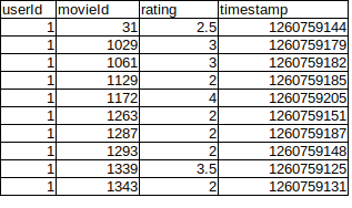
ratings_small.csv

We first read the data and get some stats about the data set:

import tensorflow as tf
import numpy as np
import matplotlib.pyplot as plt
 
#uncomment this if you're not using jupyter notebook
%matplotlib inline
 
#load the dataset
dat = np.loadtxt('ratings_small.csv', delimiter = ',', skiprows = 1)
 
#Get some stats and arrays
users = dat[:,0]
movies = dat[:,1]
ratings = dat[:,2]
users = users.astype('int32')
movies = movies.astype('int32')
uniques = [np.unique(users).shape[0], np.unique(movies).shape[0]]
print('number of unique users:', uniques[0])
print('number of unique movies:', uniques[1])
print('number of ratings:', users.shape[0])
print('total number of cells:', uniques[0] * uniques[1])
print('Ratio of entries filled:', users.shape[0]/(uniques[0] * uniques[1]))

The data set contains a bit over 9,000 movies. But the movie_id’s can be very large. So we can’t use the movie_id values as indices for our ratings matrix. However, the user_id variables range from 1 to 618. So we can use user_id as an index. Since we need to relabel the movie_ids in the range [0, 9066], we might as well sort the relabeling by the number of ratings each movie has.

"""The code below is not advised for very large dataset as many arrays are created."""
#obtain unique movie IDs
m_uniques = np.unique(movies)
 
#count the number of times that movie appears 
m_occurances = [] 
for m in m_uniques:
    occ = np.count_nonzero(movies == m)
    m_occurances.append(occ)
m_occurances = np.array(m_occurances)
 
#get the indices that sort by number of occurances.
sort_indices = np.argsort(m_occurances)
 
#The unique movie ids in descending order
m_uniques_occ_sorted = m_uniques[sort_indices]
m_uniques_occ_sorted = m_uniques_occ_sorted[::-1]
m_uniques_occ_sorted = np.array(m_uniques_occ_sorted)
 
#optionally we can also look at the occurances of movies in the dataset
m_occurances_sorted = m_occurances[sort_indices]
m_occurances_sorted = m_occurances_sorted[::-1]
 
#this plot takes some time to create.
#also the gaps in the plot are not real. They appear as artifact of trying to fit the bars into pixel sizes.
plt.figure(figsize=(10,8))
plt.bar(range(len(m_occurances_sorted[0:3000])), m_occurances_sorted[:3000])
plt.title('Number of ratings of movies')
plt.xlabel('movie_id')
plt.ylabel('Number of ratings')
plt.show()

Movie_id relabeled and sorted in descending order. This is not the full graph as it extends to 9,000

After we sort the movie_ids by number of occurrences, we can see the distribution of ratings. The movies with the most number of ratings have about 300 ratings. These are probably the Titanic and Star Wars movies. The most popular 500 movies have about 50 user ratings at least. Once we get past the 2,000th movie mark, they only have about 10 or fewer ratings. So predicting user ratings for these movies are likely going to be challenging and also very unreliable. We will see the effects of this later.

We can now generate the ratings matrix and visualize it.

M = np.zeros((uniques[0], uniques[1]))
mask = np.zeros(M.shape)
for u, m, r in zip(users, movies, ratings):
    #user ID starts from 1.
    M[u - 1, np.where(m_uniques_occ_sorted == m)[0][0]]= r
    mask[u - 1, np.where(m_uniques_occ_sorted == m)[0][0]]= 1.
     
plt.figure(figsize=(10,8))
plt.imshow(M[:,:500])
plt.xlabel('movie_id')
plt.ylabel('user_id')
plt.title('Movie ratings matrix')
plt.show()

Ratings matrix M

By design, the movies with the most number of occurrences are indexed to small numbers. So we see most ratings at the left of the matrix. We also observe that some users are power raters while others rate very sparingly. The movies are rated in the range of [0, 5].

Next we randomly mask some of the ratings to generate our validation set. We have 1M ratings, which is only 1.7% of the full matrix. So we don’t want to remove too many. In this example, I mask out 5,000 ratings. The number can be tuned with the val_count parameter.

#create validation data. We simply need to create a mask
val_count = 5000
_is = np.random.randint(0, len(users), val_count)
 
val_mask = np.zeros(M.shape)
for i in _is:
    _user = users[i] - 1
    _movie = np.where(m_uniques_occ_sorted == movies[i])[0][0]
    val_mask[_user, _movie] = 1
     
print(np.sum(val_mask))
     
plt.figure(figsize=(10,8))
plt.imshow(val_mask[:,:500])
plt.xlabel('movie_id')
plt.ylabel('user_id')
plt.title('Validation movies ratings matrix')
plt.show()

Masked out ratings. These are our target cells that we need to fill with rating predictions.

As before, I use the early stopping code. Although if you don’t use this, you can see the validation loss and training loss diverge.

def early_stopping(losses, patience = 5):
     
    if len(losses) <= patience + 1:
        return False
     
    avg_loss = np.mean(losses[-1 - patience:-1])
     
    if avg_loss - losses[-1] < 0.01*avg_loss:
        return True
     
    return False

Next, we convert the numpy matrices to tensorflow tensors. This step is not necessary, as tensorflow will do this automatically. But I highlight the code here because I’ve added an extra parameter that we can tune with. Since the ratings matrix M is sorted, we can cut it off at any point and the rejected movies will have the least ratings counts. So this means we can effectively choose to estimate matrix M based on the more popular movies. This is useful because movies with few ratings are not very reliable, nor are they very useful.

cutoff = 9000
M = tf.constant(M[:,:cutoff], dtype = 'float32')
val_mask = tf.constant(val_mask[:,:cutoff], dtype = 'float32')
train_mask = tf.constant((mask[:,:cutoff] - val_mask[:,:cutoff]), dtype = 'float32')
 
print('Number of validation ratings:', tf.reduce_sum(val_mask))
print('Number of trainign ratings:', tf.reduce_sum(train_mask))

We are now ready to apply Funk’s SVD decomposition to the ratings matrix M.

U_d = tf.Variable(tf.random.normal((671, 10)))
V_d = tf.Variable(tf.random.normal((10, cutoff)))
 
train_norm = tf.reduce_sum(train_mask)
val_norm = tf.reduce_sum(val_mask)
 
adam_opt = tf.keras.optimizers.Adam()
from datetime import datetime
lr = 0.001
ep = 0
start_time = datetime.now()
losses = []
val_losses = []
while True:
     
    with tf.GradientTape() as tape:
        M_app = U_d @ V_d
         
        pred_errors_squared = tf.square(M - M_app)
        loss = tf.reduce_sum((train_mask * pred_errors_squared)/train_norm)   
         
    val_loss = tf.reduce_sum((val_mask * pred_errors_squared)/val_norm)
 
    if ep%100 == 0:
        print(datetime.now() - start_time, loss, val_loss, ep)
        losses.append(loss.numpy())
        val_losses.append(val_loss.numpy())
    if early_stopping(losses):
        break
     
    grads = tape.gradient(loss, [U_d, V_d])
    adam_opt.apply_gradients(zip(grads, [U_d, V_d]))
 
    ep += 1
 
print('total time: ', datetime.now() - start_time)
print('epochs: ', ep)
 
plt.figure(figsize=(7,5))
plt.plot(losses, label = 'training_loss')
plt.plot(val_losses, label = 'val_loss')
plt.xlabel('training iters x100')
plt.ylabel('loss')
plt.legend()
plt.show()

Training and validation loss on ratings_small data set.

The minimum validation loss I obtained was 2.2 MSE, or about 1.5 mean error on the rating. Is this bad? May not be so bad, considering the ratings are on a 0 to 5 scale. Note that we used a latent vector size of only 10 in this decomposition. That is, (617 x 10) + (10 x 9000) variables to approximate (617 x 9000) matrix. This is a compression to about 1.7% of the original size. Also, our original matrix M was only filled to about 1.7%. Can you predict what would happen if we change latent variable size from 10 to something else?

In any case, we can try tweaking some controls to see how the validation loss changes. First, we change the latent size to see how the losses change. That is, we change U and V to [617, k] and [k, 9000] matrices, where we vary k.

Loss function as a variable of latent size

We observe above that as we increase the latent size, the error between our approximate M and real M decreases. This is expected.

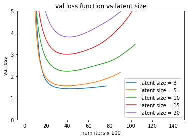
Validation loss function as a variable of latent size

However we observe that increasing the latent size actually increases validation loss. This might seem counter intuitive but this makes sense because our matrix M is so sparsely filled that increasing the latent size simply allows the U_d and V_d matrices to over fit M. By forcing the matrices to small size, we force it to generalize to M. From the plot above, our best latent size is 3, which gets about 1.5 MSE, or 1.2 real rating error. Still not ideal but not too bad.

Next, we try limiting the ratings matrix M to the more popular movies. That is, we set the cutoff points to smaller sizes. We will keep the latent size to 5 for now.

Loss function as we vary cutoff point.

Changing the cutoff point does not affect loss function too much. But cutoff does affect the validation loss.

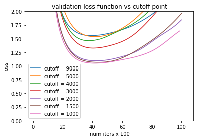
Validation loss as we vary cutoff point

We observe that we can get the validation loss to be under 1.0 if we place the cutoff point to lower than 4,000. This makes sense because the top movies have more than one or two total ratings. Therefore, each movie has more statistics and thus our error reduces. However, changing the cutoff to anything less than 4,000 does not make too much of a change. There is only so much we can approximate with such a sparsely populated rankings matrix.

Validation loss as we vary cutoff point. The latent size was increased to 10.

We can try increasing the latent size to 10. But as we see in the above figure, this makes the validation loss worse. This is again due to being able to over fit to M with more available parameters.

Conclusion

If you stuck until the end, thanks for reading. Some important discoveries made in this post are that for a matrix M of size (617, 9000), only latent size of 3 was enough to make the best approximation. This is a major reduction but we are also limited by the number of ratings available. But the important discovery is that our movie rating tendencies can be boiled down to some very small latent vectors. This is not entirely unexpected since most people will agree on which movies are good and which are bad. Our ratings prediction is better for more popular movies, going as low as mean error of about 1. Hopefully you learned something from this post.

References:

Dataset: The Movies Dataset.

Simon Funk’s original posting: link.